1 Intro

As a language, q is extremely efficient when it comes to working with vector-based data structures, and is a natural choice for all sorts of data analysis, generally far-outranking other languages when it comes to speed. Albeit recently the number of available public libraries for kdb has expanded (see https://github.com/KxSystems), often end-users find that they must create their tools to solve their problems. One of these problems is Monte-Carlo integration.

Now, we take a look at building out some code to use q to sample from distributions through several methods.

Why Sample?

In statistics, often our goal is to compute some summary of a distribution model; these summaries are essentially integrals of probability densities.

The definition of the mean and the variance of a distribution is given by the formulae:

\[\mu_{x} = \int_{x \in S} x \times f(x) dx;\] \[\sigma_{x}^2 = \int_{x \in S} (x-\mu_x)^2 \times f(x) dx;\]

where $f(x)$ is the target distribution.

In many circumstances, these summaries have closed form solutions, meaning we can analytically solve and then calculate our desired values. Take for example the Beta distribution:

\[f(x | \alpha,\beta) = \frac{\Gamma(\alpha +\beta)}{\Gamma(\alpha)\Gamma(\beta)}x^{\alpha - 1}(1 -x)^{\beta - 1}\]

where $\alpha$ and $\beta$ are the shape parameters of the function, and $\Gamma$ is the gamma function applied to the parameters.

Analytically, we can solve to find the mean and variance:

\[E(x | \alpha,\beta) = \frac{\alpha}{\alpha + \beta}\] \[Var(x | \alpha,\beta) = \frac{\alpha\beta}{(\alpha + \beta)^2 (\alpha + \beta +1) }\]

but, what if we had a function that we couldn’t solve analytically? In cases like these, we turn to sampling. The logic of sampling is that we can generate (simulate) a sample of size $n$ from the distribution of interest and then use discrete formulas applied to these samples to approximate the integrals of interest, i.e the above equations become:

\[\mu_{x} = \int_{x \in S} x \times f(x) dx \approx{\frac{1}{n} \sum_{x \in S} x}\] \[\sigma_{x}^2 = \int_{x \in S} (x-\mu_x)^2 \times f(x) dx \approx{\frac{1}{n} \sum_{x \in S} (x-\mu_x)^2}\]

Random Number Generation

To use the simulation-based techniques described in this blog, we will need to be able to generate sequences of random numbers from the uniform distribution. To do this in q, we can use the ?[x;y] overload. Where x is the number of samples and y is the maximum value of a single sample. A negative x is interpreted as generate a random number without replacement. The result also depends on the data type of y, i.e

// Generate 10 longs
q)10 ? 20
14 6 7 4 6 10 9 9 10 18

// Generate 10 floats
q)10 ? 20f
17.79407 2.139848 8.444447 15.34972 17.70322 8.717351 1.55764 8.467533 12.45664 3.944245

// Generate 10 longs without replacement
q)-10?10
7 1 3 9 5 0 4 6 8 2
// Cannot do the following:
q)-11?10
'length

q)-1?10.
'type

Pseudo-Random Number Generator (PRNG)

Along with most other analytics software, q does not generate genuine random numbers. Instead, pseudo-random numbers are generated that appear to be random but are actually deterministic. The implication of this is a topic of its own, but it’s important to understand that we can choose the initial seed via the command line parameter \S(https://code.kx.com/q/basics/syscmds/#s-random-seed). This displays or sets the initial seed for the PRNG. Resetting the seed to the default value allows the pseudo-random values to be reproduced, i.e:

q)a: 1000?10
q)\S
-314159i
// Resetting \S
q)\S -314159i
q)b: 1000?10
q)a~b
1b

Generation of random numbers natively in q is limited to the uniform distribution, in this blog, we extend this to non-uniform distributions.

Visualisation Libraries

To recreate the visualisations, and to use the mcplot.q script, we utilise the Kx Developer implementation of ‘grammar of graphics’ libraries. Functional reference and instructions can be found here: https://code.kx.com/developer/libraries-setup/

2 Transformation Based Methods

Transformation based sampling are those where we map a uniform random sample into a random sample of a given distribution based on rules related to the target distribution.

2.1 Inverse Sampling

The most basic method (but not always the easiest to achieve) is inverse sampling, it essentially follows 2 steps:

1. Draw a uniform random number $u$ between 0 and 1.
   • $u \sim U(0,1)$
2. then $z= F^{-1}(u)$ is draw from $f$.
   • where $F(x) = \int f(x)$, the CDF of the function

This works because $F(z)$ varies between 0 and 1, and inverting $F \rightarrow F^-1$ allows us to use the uniform input and return a value according to the original distribution.

Example 1: Linear Density Function

Lets take a sample linear function such as:

\[f(x) = (1/40)(2x+3);\space \space\space \space 0 \le x \le 5\]

Plotting the distribution:

lin:{(1%40)*3+2*x};
xs:(1+ til 100)%20;
ys: lin xs;
t:([] fx:ys;x:xs);

.qp.png[`fig1.png;500;500]
    .qp.theme[@[.gg.theme.transparent;`marker_default_fill;:;.gg.colour.LightSteelBlue]] 
    .qp.area[t;`x;`fx;::]

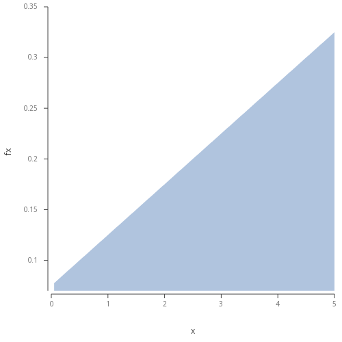Figure 1 - Basic area plot of the described linear function.

In order to generate samples from the distribution, we need to generate $u = U(0,1)$ and compute $z$ that satisfies $u=∫_0^z (1/40)(2x+ 3)dx$.

This is readily solvable to

\[z=−3+\sqrt{160u+ 92}\]

We can then look to generate samples through some basic code

// Create wrapper to take in a function and number of iterations
.mc.inv:{[fn;n]
            fn n?1.
            };
// Inverse of the integral of our function
Finv:{0.5*-3+sqrt 9+160*x};
sp:.mc.inv[Finv;1000];

2.693191 2.186069 4.520798 3.094167 4.527468 0.4514672 0.741578 2.9123 2.587419 3.492536 1.466129 0.1019155 4.119329 3.423405 4.641388 1.43545 3.814846 3.034265 2.294017 1.696239 2.105466 3.283129 1.099786 2.346678 4.171379 2.717967 3.589762 1.208051 1.551293 0.4776696 0.264516 3.867128 3.357385 0.3302062 1.994477 1.461246 4.184818 4.662508 3.547179 3.59022 4.172732 1.775157 3.901211 3.87638 4.520041 1.85951 0.1526045 3.777172 3.008494 4.389643 0.3466325 2.009075 4.790601 3.643624 4.415163 1.811094 0.2489897 3.457904 2.019989 4.158845 3.143862 4.991487 3.646076 4.94719 4.948074 4.729302 3.753599 2.634288 3.739414 4.963077 3.363908 4.609675 2.686786 3.868926 4.311823 3.252548 4.231208 1.472318 4.893727 1.150462 3.284663 3.492756 4.822941 4.552986 1.552536 4.311677 3.387747 3.952968 2.725551 4.310725 3.24897 1.541481 4.919932 4.830202 4.017228 1.41601 3.717564 2.423435 4.102193 0.446528 3.269507 4.450899 1.803247 0.8132367 4.218201 2.170766 2.103313 3.040327 4.545846 4.356087 4.513533..

We can then use some regular keywords to work out the standard deviation and the mean.

q)avg sp
3.022665
q)sdev sp
1.358939

What about the overall distribution of the samples? Does it match the original function that we sampled from? We can generate a histogram to visualise the distribution.

A basic line of code that will produce a histogram in the form of a dictionary is below; bucketing the data into segments of width 0.5.

(!). flip distinct  g,'(count; sp) fby g:0.5 xbar sp

A similar function is built into the q-ggplot implementation, available via .qp.hist. Some wrapper functions, shown in this blog, exist in the mcplot.q script, these are simple tools to help plot and fit the data that’s explored. Here we fit the histogram of our samples to the original function:

/width of histogram bins
w:0.1;
.mc.plot.fitHist.png[sp;lin;w;1b;`large;`fig2.png]

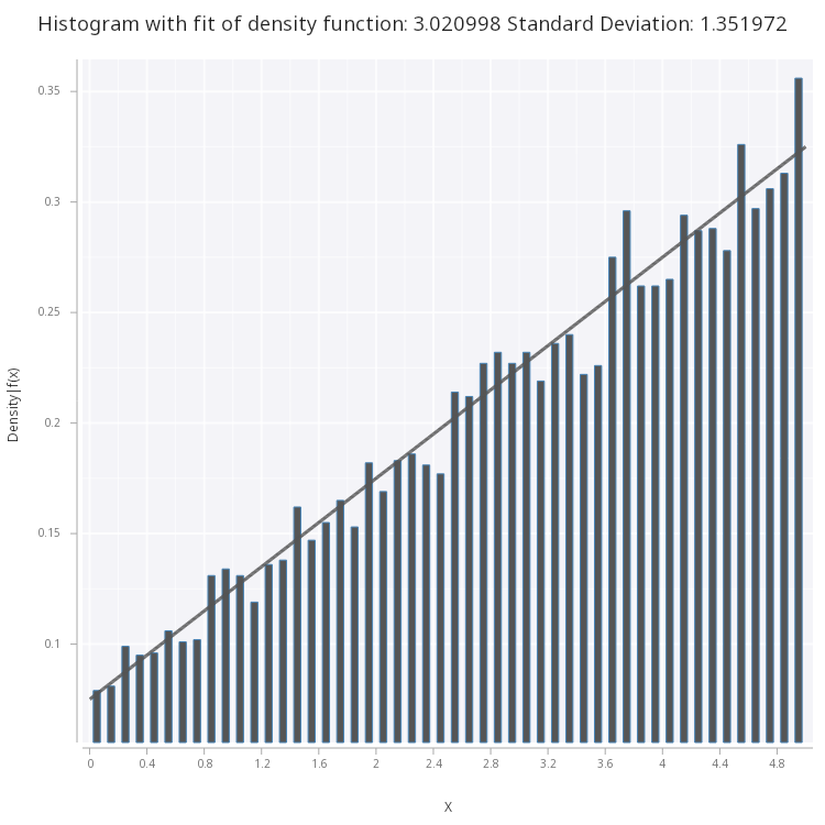Figure 2 - Linear Density Function fitted on histogram of the samples.

From what we can see, our original function is a good fit for the histogram, however, there are more statistically sound methods of determining goodness-of-fit, outside the scope of this blog, such as the chi-squred test.

Another example of this is the exponential function, with

\[f(x) = {\lambda}e^{-{\lambda}x}\]

Which has a CDF:

\[F(X) = 1-e^{-x\lambda}\]

and the inverse CDF:

\[F^{-1}(u) = -\frac{\log(1-u)}{\lambda}\]

Following the first example, we can generate some samples with a specific parameter, below is the code for $\lambda = 2$

/exponential PDF
expF:{y*exp neg[x*y]};
/lambda = 2
expF2:expF[;2];
/ inverse CDF
invExpF:{log[1-x]%neg[y]};
/lambda =2
invExpF2:invExpF[;2];

// Generate 100000 samples
sp:.mc.inv[invExpF2;100000];

Analytically, it can be shown that the mean and standard deviation of the exponential distribution is $\sigma =\mu = \frac{1}{\lambda}$. We can see that when we inspect the samples, this matches our expectations.

q)avg sp
0.4994483
q)sdev sp
0.4990704

Plotting this, we see that the pdf correctly fits the sample histogram

.mc.plot.fitHist.png[sp;expF2;0.1;1b;`medium;`fig3.png]

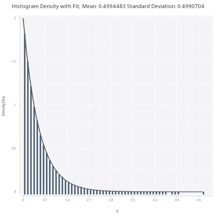Figure 3 - Exponential Density Function fitted on histogram of the samples.

We see that the inverse function is trivial to implement in q, and it is very efficient at generating samples - however, there are major drawbacks to this method. For one, if the CDF is not analytically solvable, this method cannot be used. For example, the normal distribution cannot be directly solved. The other problem with this is that we require our density to be normalised, unlike what we will see with rejection and importance sampling, this is a strict requirement for inverse sampling.

2.2 Box-Muller Transform

We mentioned that the inverse transform method does not work for the normal distribution, thankfully there is another transformation method which can accurately and efficiently generate normally distributed samples, it is called the Box-Muller Method. The basic method follows below:

1. Generate a pair of independent uniform variables $U_1, U_2$

2. Calculate independent normal samples $~\mathcal{N}(0,1),$ $Z_1,Z_2$ via:

   \[Z_1 = \sqrt{-2\log U_1}\cos(2\pi\, U_2)\\ Z_2 = \sqrt{-2\log U_1}\sin(2\pi\, U_2)\]
3. Sampling with non-unit mean and standard deviation $\mu, \sigma$ :

\[x = \sigma Z+\mu\]

Building this out in q is fairly simple, in our code we supply a parameter n to dictate the number of samples generated and use this number to take from both $Z_1$ and $Z_2$ :

.mc.pi:acos -1;
.mc.norm.bxml:{[n;s;m]
    u1:(c:ceiling[n%2])?1.;
    u2:c?1.;
    m+s*n#(sqrt[-2*log(u1)]*cos 2*.mc.pi*u2),sqrt[-2*log(u2)]*sin 2*.mc.pi*u1
    };

Following the previous examples, we see that the code generates accurately distributed samples:

q)sp:.mc.norm.bxml[1000000;3;0.5];
q)avg sp
0.4999065
q) sdev sp
3.001964

We see plot and fit the normal distribution to the histogram of the samples:

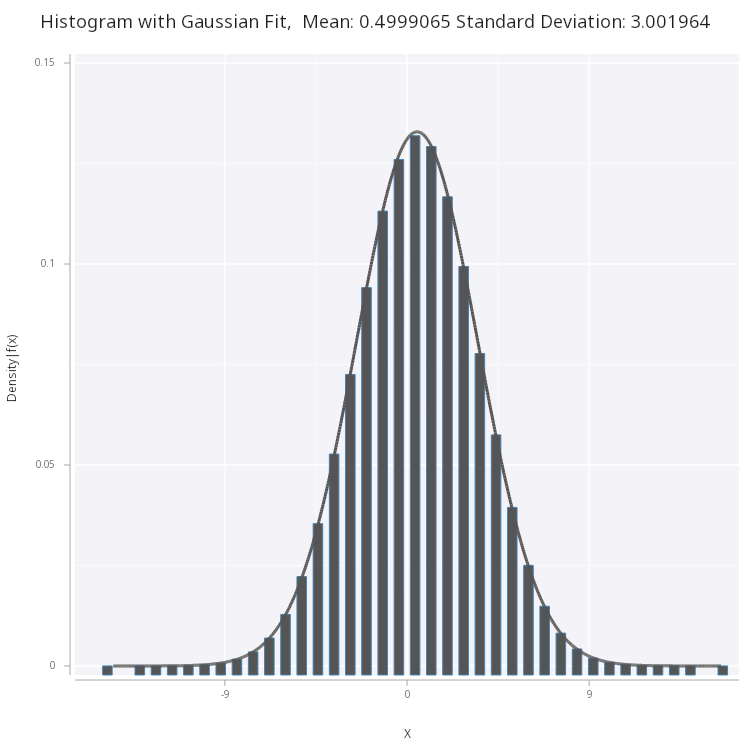Figure 4 - Normal PDF fitted on histogram of the samples generated via box-muller method.

The Box-Muller method is an efficient way of generating normally distributed samples. As we will further on, generating normally distributed samples will act as a starting point when sampling from other distributions.

We can also use our samples to roughly estimate other values such as the probability between two values, x at a given probability, and also the inverse of the PDF. Below are some utility functions that determine:

• The probability p of outcomes between a range y and z.
• Given a probability p and starting point y, the value closest value to z.
• Given the output of a symmetrical function like the normal PDF, the resulting input x.

.mc.util.spInt:{(count where x within(y;z))%count[x]}

.mc.util.spIntInv:{[x;y;p]
   x where d=min abs d:p-.mc.util.spInt[x;y;] each x: asc x;
    };    
    
.mc.util.symInv:{ 
    n: (floor count[x]%2) cut m:.mc.norm.fn[sdev x;avg x;] x:asc x;
    if[3~ count n; n:(n[0];n[1],n[2])];
     x where m in  raze n ./:  0 1,' where each abs[d]=' min each abs d: n - y
    };

For example, we can integrate between 0 and 1:

q)sp:.mc.norm.bxml[200000;1;0];
q).mc.util.spInt[sp;0;1]
0.34161

Or given a probability 0.5:

q).mc.util.spIntInv[sp;-10;0.5]
0.01032863

Find the two points where y = 0.4

q).mc.util.symInv[sp;0.4]
-0.0008748167 -0.0007929524

3 Rejection Sampling

Transformation based methods provide efficient ways to sample from distributions that we can analytically derive the generator functions. However, as we have seen these basic methods fall short when trying to sample from distributions that cannot be analytically resolved. Rejection sampling provides a powerful (albeit inefficient) way to sample from any distribution.

Sampling from a distribution $f(x)$ involves three basic steps:

1. Sample a value $z$ from a distribution $g(x)$ from which we can easily sample from. The requirement is that at all point $m\times g(x)$ is greater than $f(x).$ Where $m$ is a constant.
2. Compute the ratio $R = \frac{f(x)}{m\times g(x)}$.
3. Compare $R$ against a uniformly distributed sample $u∼U(0,1)$. If $R>u$, then we accept $z$ as a draw from $f(x)$. Otherwise reject $z$.

The intuition behind this is as follows. We have a function $g(x)$ which (after being multiplied by a constant) should completely envelope the target function $f(x)$. The sample $z$ from $g(x)$ provides a value on the x-axis for the potential sample. We evaluate $m\times g(z)$, which gives us a value on the y-axis. We generate $u∼U(0,1)$ because in essence we are actually considering whether $m\times g(z) \times u<= f(z)$. This is equal to drawing from $U(0,m\times g(z))$ and seeing whether the value is within $f(z)$. The below diagram explains how this works:

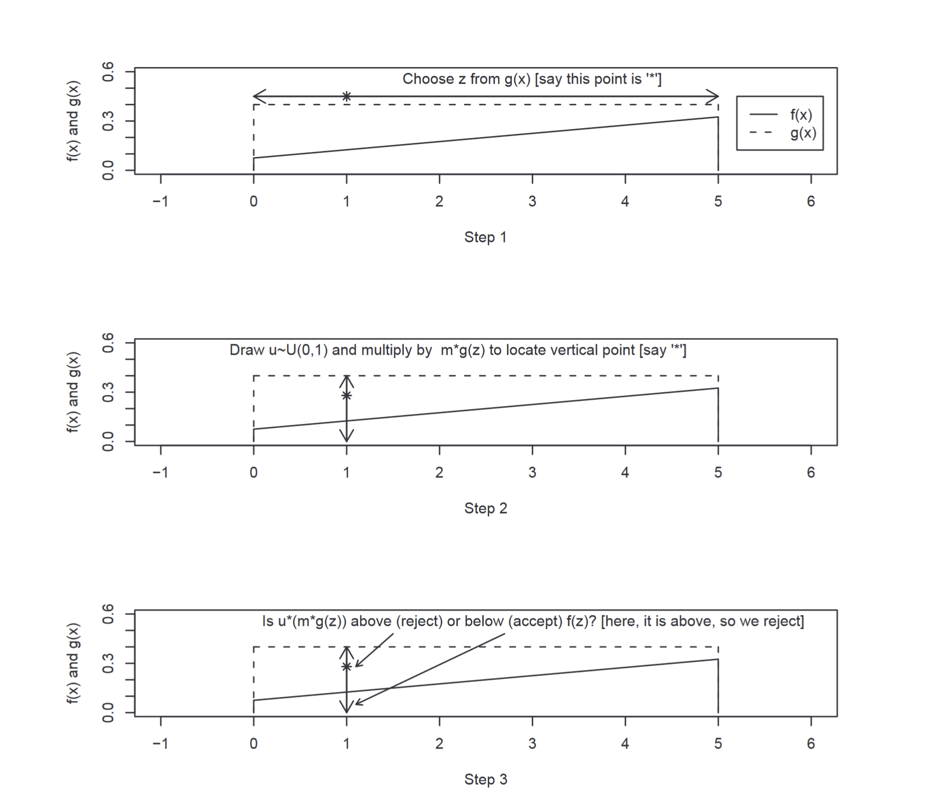Figure 5 - Step through rejection sampling (Scott M. Lynch)

It’s important to note that the choice envelope function is one that should cover the entire range of possible values of the target distribution. The uniform distribution is often a good choice as it has a very predictable acceptance rate and can be customized to cover the desired distribution. This predictability is important because we can use the information for the total number of samples utilize vector computation in q, instead of having to investigate each sample one-by-one.

The drawback comes when drawing from distributions with infinite range, such as the normal distribution, as there is no corresponding $U(-\inf,\inf)$. In these cases, we can either approximate with a large tail approximation or to use an envelope function with infinite support.

The below set of function sets up a generalised rejection sampler.

.mc.i.rejsp:{[n;m;h;fn;s;e;x] 
    x,y where(fn y:s+n?"f"$e-s)>n?m*h
    };

.mc.rej.sph:{[fn;n;s;e;h;m]
    // rejection sampling
    // fn : target function
    // n: number of samples
    // s: lower limit
    // e: upper limit
    // m: envelop function multiple
    // h: 
    $[not h;
        h:max fn .mc.utils.linspace[s;e;10000];
        h:1%(e-s)
        ];
    if[not m;
        m:1.001
        ];
    / n2 = estimate of total iterations needed to get n samples,
    // multiplied by 1.1 to reduce chance of rerun.
    n2:ceiling 1.1* n*(e-s)*m*h;
    n#.mc.i.rejsp[n2;m;h;fn;s;e]/[n > count@;()]
    };
    
.mc.rej.sp:.mc.rej.sph[;;;;0b;0b];

The routine works by assuming a total number of samples required based on the ratio of the envelop and target distribution, then we can select the samples that fall within the right value - if there are not enough samples (which is unlikely) then it can be run again one more time.

Returning to the previous examples with the linear density function, in a few seconds we can generate 10 million samples:

q)\t sp:.mc.rej.sp[lin;10000000;0;5];
3421
q)avg sp
3.020848
q)sdev sp
1.346187

The limitation with this routine comes to play with sampling from normal or exponential distribution - we have to set a limit on what can be sampled, which will reduce the accuracy of our estimates. The workaround would be to write an ad-hoc rejection code with the desired envelope function. Exponential with 0, 10 start and endpoint:

q)sp:.mc.rej.sp[expF2;1000000;0;10]
q)avg sp
0.4998324
q)sdev sp
0.499901

Normal with -10, 10 start and end point:

sp:.mc.rej.sp[.mc.norm.fn[1;0;];100000;-10;10];
q)avg sp
0.002640996
q)sdev sp
1.00329

We see that with some adjustment and understanding of the limitations, we can use rejection sampling to sample from any distribution. Rejection and transformation sampling are basic methods that often work as the basis for more sophisticated and efficient Monte-Carlo methods. We will see in future series how these make up the foundation of Monte-Carlo Markov Chain algorithms.

4 Importance Sampling

In rejection sampling, one of the main downfalls is the inefficiency involved with having to reject samples that fall outside the domain of the target distribution - but what if there was a way of utilizing all the samples that are generated instead of discarding them? There exists a method that does just that, called importance sampling.

Importance Sampling is not sampling as compared to the previous methods. In fact, in Importance Sampling, we are not directly sampling from a target distribution, but instead generating samples from a different distribution and calculates properties for the target distribution based on the samples. In this method, the samples produced are not of interest — only are the properties derived from them.

The idea is that we want to find properties of a function $h(x)$ where $x$ is distributed according to our target distribution $f(x)$. We know that

\[\mathbb{E_f[h(x)]} = \int h(x)f(x)dx\\ \approx \frac{1}{N}\sum_{i}^{N}h(x_i)\]

But as we’ve seen before, it may be hard to directly sample from the target distribution. In these cases, we can use a proposal distribution $g(x)$ which covers the domain of the target distribution. We apply a weight to the samples from this proposal distribution to determine how ‘under’ or ‘over’ represented they are compared to the target distribution. The maths that follows:

\[\mathbb{E_f[h(x)]} = \int h(x)f(x)dx =\int h(x)\frac{f(x)}{g(x)}g(x)dx =\mathbb{E_g[h(x)\frac{f(x)}{g(x)}]}\]

What we see is that if we can calculate the ratio between the two distributions, called the importance weights $w(x)$ it can give us our estimated mean:

\[\mu_n = \frac{1}{n}\sum_{i=1}^n\frac{f(x_i)}{g(x_i)}h(x_i) = \frac{1}{n}\sum_{i=1}^n w_i h(x_i) \approx \mathbb{E}_f[h(X)]\]

In essence, we are taking $x$ generated from $g(x)$ and ‘reweighing’ them before taking the average. Importantly, we can extend this to work with normalized distributions, and it can be shown that the addition of a normalising factor brings our equation to:

\[\mu_n =\frac{\frac{1}{n}\sum_{i=1}^n w_i h(x_i)}{\frac{1}{n} \sum_{i=1}^n w_i}\]

Importance Sampling is often used as a variance reduction method of estimation - this means that the total number of samples required to estimate the mean with small enough variance is less than other Monte-Carlo methods, in addition to the fact that all samples are used in determining the output, makes this a very powerful technique. The fact that we can sample values for a function of $x$ i.e $h(x)$, means that we can calculate more than just the mean. For example, the standard deviation is given by:

\[\sigma^2 = \mathbb{E[x^2]} -\mathbb{E[x]}^2\]

We can use the substitute $x^2=h(x)$ in the second part of the above formula to get the standard deviation of the desired distribution.

Importance sampling code

The basic algorithm follows:

1. Draw $x_1, x_2,…x_n$ from proposal distribution $g(x)$.
2. Calculate the importance weights $w_i = \frac{f(x_i)}{g(x_i)}$.
3. Estimate the average $\mu = \frac{\sum_i w_i h(x_i)} {\sum_i {w_i}}$.

In the following code, we use the normal distribution as a default proposal if one is not given in the o parameter. The code will by default return the mean and the standard error (of the mean), optionally the standard deviation (of the target) can be returned as well.

.mc.i.impCalcNorm:{[x;f;g;h]
    x:(h[x]*w:f[x]%g[x]);
    :(avg[x]%avg w;sdev[x]%sqrt[count x])
    };

.mc.imp.spn:{[f;h;n;o]
    /f - target density
    /h - function on x
    /n - number of samples
    /o - options dictionary `std`g`s!(1b/0b; custom g[x]; samples from g[x])
    if[0b~o;o:()!()];
    o:(``std`g`s!raze(::;3#0b)),o;
    if[(0> type o[`s])<>100>type o[`g]; 0N!"ERROR - Incorrect g/o arguments supplied";:()];
    if[0b~o`g;
            o[`s]:.mc.norm.bxml[n;1;0];
            o[`g]:.mc.norm.fn[1;0;]
        ];
    o[`avg`sderr]:.mc.i.impCalcNorm[o`s;f;o`g;h];
    if[o`std;
        o[`std]: sqrt first[.mc.i.impCalcNorm[o`s;f;o`g;{y[x] xexp 2}[;h]]] - xexp[o`avg; 2 ]
        ];
    `s`g _ o
    };

In the below example we estimate from a target guassian distribution with $\mu = \sigma = 1$ and the proposal is the standard normal:

q)options:((),`std)!(),1b;
q).mc.imp.spn[f:.mc.norm.fn[1;1;];{x};1000;options];
std  | 0.9673603
avg  | 0.9855257
sderr| 0.09516791

We see that we can get a seemingly accurate result with only 1000 iterations. The choice of proposal distribution is important, in the next example we see that using the above proposal does not lead to great results for a distribution with $\mu = 5, \sigma = 1$:

q).mc.imp.spn[f:.mc.norm.fn[1;5;];{x};10000000;options];
std  | 0.6498159
avg  | 4.446898
sderr| 0.5324564

To combat this, we can provide a custom proposal function and it’s samples, below uses samples from a uniform proposal covering -10 to +10:

q)s:-10;
q)e:10;
/ uniform function
q)fn:{[s;e;x] $[x within(s;e);1%(e-s);0]}[s;e] each;
/samples
q)sp:.mc.uni.sp[s;e;1000];
q)options:(`std`g`s)!(1b;fn;sp);
q).mc.imp.spn[f:.mc.norm.fn[1;5;];{x};1000;options]
std  | 0.9699811
avg  | 4.966861
sderr| 0.3537732

We see that even with 1000 samples when we choose a better proposal distribution, our output is much more accurate. Importance Sampling can be used to greatly reduce the number of required samples.

5 Conclusion

In this blog, we laid the foundations for sampling. We looked at transformation methods of sampling, where after an analytical transformation of the distribution. Transformations have strict requirements for being able to analytically derive something from the original PDF, in cases where this is impossible we turned to rejection sampling. In theory, rejection sampling should be able to sample from any distribution, although it has its drawbacks, one being the inefficiency in having to reject samples that don’t fall within the target distribution. Finally, we looked at importance sampling which alleviated the rejection problem, however, this method also came with its drawback in having to carefully select the best proposal distribution for accurate results.

This will be one part of a multi-part blog series. In the next iteration, we will look to implement Monte-Carlo-Markov-Chain (MCMC) methods in q. These methods utilize the basic sampling methods as the building blocks.

6 References

1. Introduction to Applied Bayesian Statistics and Estimation for Social Scientists (Scott M. Lynch)
2. Advanced Statistical Computing (Roger D. Peng https://bookdown.org/rdpeng/advstatcomp/)
3. Importance Sampling Introduction https://towardsdatascience.com/importance-sampling-introduction-e76b2c32e744
4. Rejection Sampling https://en.wikipedia.org/wiki/Rejection_sampling
5. Monte Carlo theory, methods, and examples (Art Owen, https://statweb.stanford.edu/~owen/mc/)